42 how to add data labels to a pie chart in excel on mac
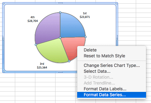
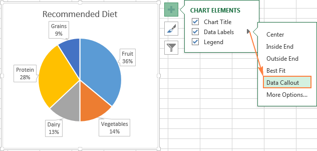
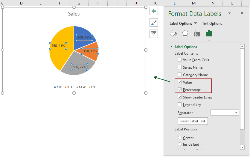
› graphs › pie-chartsFree Pie Chart Maker - Make a Pie Chart in Canva Skip the complicated calculations – with Canva’s pie chart generator, you can turn raw data into a finished pie chart in minutes. A simple click will open the data section where you can add values. You can even copy and paste the data from a spreadsheet. Click the text to edit the labels. Pie Chart in Excel | How to Create Pie Chart - EDUCBA Step 4: Select the data labels we have added and right-click and select Format Data Labels. Step 5: Here, we can so many formatting. We can show the series name along with their values, percentages. We can change these data labels' alignment to center, inside end, outside end, Best fit. Step 6: Similarly, we can change the color of each bar ...
Change the look of chart text and labels in Numbers on Mac If you can't edit a chart, you may need to unlock it. Change the font, style, and size of chart text Edit the chart title Add and modify chart value labels Add and modify pie chart wedge labels or donut chart segment labels Modify axis labels Edit pivot chart data labels Note: Axis options may be different for scatter and bubble charts.

How to add data labels to a pie chart in excel on mac
How to format the data labels in Excel:Mac 2011 when showing a ... Try clicking on Column or Row you want to set. Go to Format Menu Click cells Click on Currency Change number of places to 0 (zero) (if in accounting do the same thing. _________ Disclaimer: The questions, discussions, opinions, replies & answers I create, are solely mine and mine alone, and do not reflect upon my position as a Community Moderator. How to Create a Graph in Microsoft Word - Lifewire 09.12.2021 · In the Excel spreadsheet that opens, enter the data for the graph. Close the Excel window to see the graph in the Word document. To access the data in the Excel workbook, select the graph, go to the Chart Design tab, and then select Edit Data in Excel. support.microsoft.com › en-us › officeAdd or remove data labels in a chart - support.microsoft.com For example, in the pie chart below, without the data labels it would be difficult to tell that coffee was 38% of total sales. Depending on what you want to highlight on a chart, you can add labels to one series, all the series (the whole chart), or one data point. Add data labels. You can add data labels to show the data point values from the ...
How to add data labels to a pie chart in excel on mac. › charts › progProgress Doughnut Chart with Conditional Formatting in Excel Mar 24, 2017 · Step 2 – Insert the Doughnut Chart. With the data range set up, we can now insert the doughnut chart from the Insert tab on the Ribbon. The Doughnut Chart is in the Pie Chart drop-down menu. Select both the percentage complete and remainder cells. Go to the Insert tab and select Doughnut Chart from the Pie Chart drop-down menu. How to add data labels from different column in an Excel chart? Right click the data series in the chart, and select Add Data Labels > Add Data Labels from the context menu to add data labels. 2. Click any data label to select all data labels, and then click the specified data label to select it only in the chart. 3. Actual vs Targets Chart in Excel - Excel Campus 04.11.2019 · I also wanted to show you that you can add data labels to your chart in order to show: Values Percentage of Target . Learn more about how to go about that from this tutorial. Variance. If you are interested in learning more about variance, I recommend this tutorial: Variance on Clustered Column or Bar Chart. Conclusion. Charting an actual number in the … EOF
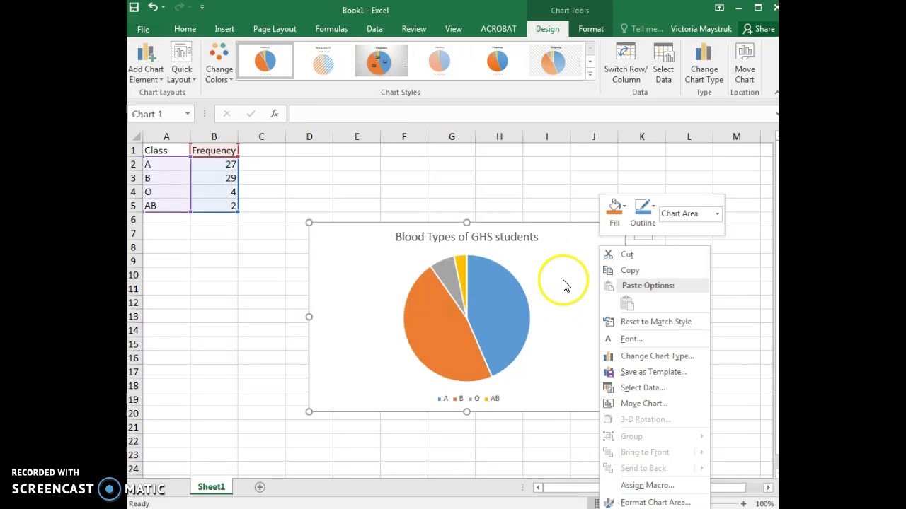
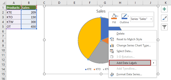
Microsoft Excel Tutorials: Add Data Labels to a Pie Chart - Home and Learn To add the numbers from our E column (the viewing figures), left click on the pie chart itself to select it: The chart is selected when you can see all those blue circles surrounding it. Now right click the chart. You should get the following menu: From the menu, select Add Data Labels. New data labels will then appear on your chart: Progress Doughnut Chart with Conditional Formatting in Excel 24.03.2017 · Step 2 – Insert the Doughnut Chart. With the data range set up, we can now insert the doughnut chart from the Insert tab on the Ribbon. The Doughnut Chart is in the Pie Chart drop-down menu. Select both the percentage complete and remainder cells. Go to the Insert tab and select Doughnut Chart from the Pie Chart drop-down menu. › 762481 › how-to-make-a-pie-chartHow to Make a Pie Chart in Google Sheets - How-To Geek Nov 16, 2021 · On the Setup tab at the top of the sidebar, click the Chart Type drop-down box. Go down to the Pie section and select the pie chart style you want to use. You can pick a Pie Chart, Doughnut Chart, or 3D Pie Chart. You can then use the other options on the Setup tab to adjust the data range, switch rows and columns, or use the first row as headers. How to show percentage in pie chart in Excel? - ExtendOffice Select the data you will create a pie chart based on, click Insert > I nsert Pie or Doughnut Chart > Pie. See screenshot: 2. Then a pie chart is created. Right click the pie chart and select Add Data Labels from the context menu. 3. Now the corresponding values are displayed in the pie slices.
How to Make a Pie Chart with Multiple Data in Excel (2 Ways) - ExcelDemy Steps: First, select the entire data set and go to the Insert tab from the ribbon. After that, choose Insert Pie and Doughnut Chart from the Charts group. Afterward, click on the 2nd Pie Chart among the 2-D Pie as marked on the following picture. Now, Excel will instantly create a Pie of Pie Chart in your worksheet. How to display leader lines in pie chart in Excel? - ExtendOffice To display leader lines in pie chart, you just need to check an option then drag the labels out. 1. Click at the chart, and right click to select Format Data Labels from context menu. 2. In the popping Format Data Labels dialog/pane, check Show Leader Lines in the Label Options section. See screenshot: 3. How to add axis labels in Excel Mac - Quora Answer (1 of 6): Click the chart, then click the Chart Layout tab. Under Labels, click Axis Titles, point to the axis that you simply want to add titles to, then click the choice that you simply want. Select the text within the Axis Title box, then type an axis title. For more Shortcuts, tricks,... Broken Y Axis in an Excel Chart - Peltier Tech 18.11.2011 · Add the secondary horizontal axis. Excel by default puts it at the top of the chart, and the bars hang from the axis down to the values they represent. Pretty strange, but we’ll fix that in a moment. Format the secondary vertical axis (right of chart), and change the Crosses At setting to Automatic. This makes the added axis cross at zero, at the bottom of the chart. (The …
Change the format of data labels in a chart
Add or remove data labels in a chart - support.microsoft.com For example, in the pie chart below, without the data labels it would be difficult to tell that coffee was 38% of total sales. Depending on what you want to highlight on a chart, you can add labels to one series, all the series (the whole chart), or one data point. Add data labels. You can add data labels to show the data point values from the ...

Change the format of data labels in a chart
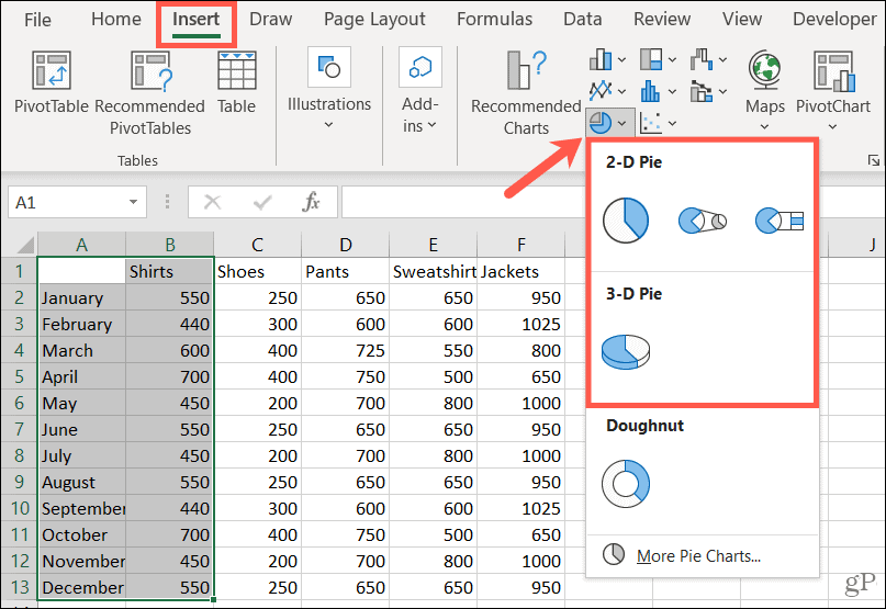
› Make-a-Pie-Chart-in-ExcelHow to Make a Pie Chart in Excel: 10 Steps (with Pictures) Apr 18, 2022 · Click the "Pie Chart" icon. This is a circular button in the "Charts" group of options, which is below and to the right of the Insert tab. You'll see several options appear in a drop-down menu: 2-D Pie - Create a simple pie chart that displays color-coded sections of your data. 3-D Pie - Uses a three-dimensional pie chart that displays color ...
How to Make a Pie Chart in Excel
How to Make a Pie Chart in Google Sheets - How-To Geek 16.11.2021 · For pie charts in particular, you have two additional sections to work with: Pie Chart and Pie Slice. These areas let you customize your pie exactly as you like. Under Pie Chart, add and adjust a doughnut hole in the center or choose a border color for the pie. You can then add labels to the individual slices if you like. You can pick from ...

How to Make a Pie Chart in Excel - All Things How
Free Pie Chart Maker - Make a Pie Chart in Canva Pie chart maker features. With Canva’s pie chart maker, you can make a pie chart in less than a minute. It’s ridiculously easy to use. Start with a template – we’ve got hundreds of pie chart examples to make your own. Then simply click to change the data and the labels. You can get the look you want by adjusting the colors, fonts ...
Change the format of data labels in a chart
Excel custom pie chart labels - Microsoft Community Excel custom pie chart labels. I want to use a pivot table to make a pie chart out of this. I want each of the pieces of the pie to contain the number of entries and between parentheses the percentage. So in the "Yes" piece, there should be '3 (33%)'. Actually, if I hover the pie chart in Excel, I get exactly the notation O want!

Directly Labeling Excel Charts - PolicyViz
How to Create and Format a Pie Chart in Excel - Lifewire To add data labels to a pie chart: Select the plot area of the pie chart. Right-click the chart. Select Add Data Labels . Select Add Data Labels. In this example, the sales for each cookie is added to the slices of the pie chart. Change Colors

Optimally positioning pie chart data labels in Excel with VBA ...
How to Make a Pie Chart in Excel & Add Rich Data Labels to The Chart! Creating and formatting the Pie Chart. 1) Select the data. 2) Go to Insert> Charts> click on the drop-down arrow next to Pie Chart and under 2-D Pie, select the Pie Chart, shown below. 3) Chang the chart title to Breakdown of Errors Made During the Match, by clicking on it and typing the new title.

How to Create a Pie Chart in Excel | Smartsheet
How to create a chart in Excel from multiple sheets - Ablebits.com 29.09.2022 · 3. Add more data series (optional) If you want to plot data from multiple worksheets in your graph, repeat the process described in step 2 for each data series you want to add. When done, click the OK button on the Select Data Source dialog window. In this example, I've added the 3 rd data series, here's how my Excel chart looks now: 4 ...
How to Create a Pie Chart in Excel | Smartsheet
How to make a Gantt chart in Excel - Ablebits.com 30.09.2022 · 3. Add Duration data to the chart. Now you need to add one more series to your Excel Gantt chart-to-be. Right-click anywhere within the chart area and choose Select Data from the context menu.. The Select Data Source window will open. As you can see in the screenshot below, Start Date is already added under Legend Entries (Series).And you need to add …

How to show percentage in pie chart in Excel?
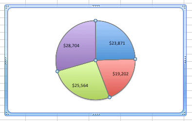
Change the format of data labels in a chart Data labels make a chart easier to understand because they show details about a data series or its individual data points. For example, in the pie chart below, without the data labels it would be difficult to tell that coffee was 38% of total sales. You can format the labels to show specific labels elements like, the percentages, series name, or category name.
How to make a pie chart in Excel
› office-addins-blog › create-chartHow to create a chart in Excel from multiple sheets Sep 29, 2022 · 3. Add more data series (optional) If you want to plot data from multiple worksheets in your graph, repeat the process described in step 2 for each data series you want to add. When done, click the OK button on the Select Data Source dialog window. In this example, I've added the 3 rd data series, here's how my Excel chart looks now: 4.
Add data labels to pie chart and delete legend
support.microsoft.com › en-us › officeChange the format of data labels in a chart To get there, after adding your data labels, select the data label to format, and then click Chart Elements > Data Labels > More Options. To go to the appropriate area, click one of the four icons ( Fill & Line , Effects , Size & Properties ( Layout & Properties in Outlook or Word), or Label Options ) shown here.
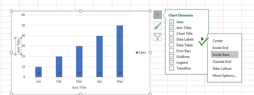
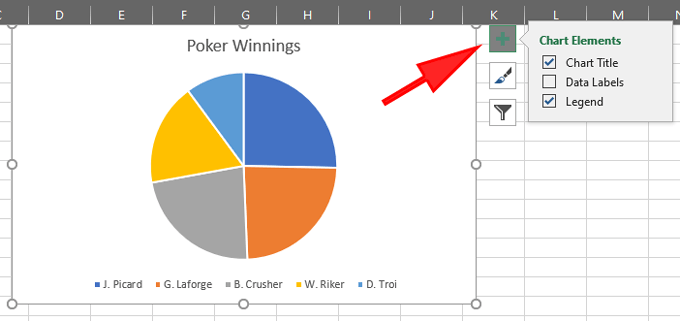
How to Add and Remove Chart Elements in Excel
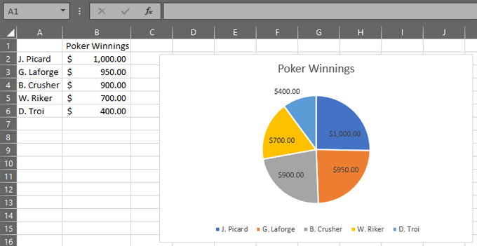
Building Pie Charts | Microsoft Excel for Mac - Basic Creating a Pie Chart. Select A7:B8; Go to Insert --> Recommended Charts and select the pie chart; Adding context. Select the chart title, press the equals key, click on A4 and press Enter; Click on the pie chart; Right click and choose Add Data Labels; Right click the Data Labels and choose Format Data Labels; Select Percentage and clear the Values
How to Create a Pie Chart in Excel | Smartsheet
support.microsoft.com › en-us › officeAdd or remove data labels in a chart - support.microsoft.com For example, in the pie chart below, without the data labels it would be difficult to tell that coffee was 38% of total sales. Depending on what you want to highlight on a chart, you can add labels to one series, all the series (the whole chart), or one data point. Add data labels. You can add data labels to show the data point values from the ...

Change the format of data labels in a chart
How to Create a Graph in Microsoft Word - Lifewire 09.12.2021 · In the Excel spreadsheet that opens, enter the data for the graph. Close the Excel window to see the graph in the Word document. To access the data in the Excel workbook, select the graph, go to the Chart Design tab, and then select Edit Data in Excel.
How to show percentage in pie chart in Excel?
How to format the data labels in Excel:Mac 2011 when showing a ... Try clicking on Column or Row you want to set. Go to Format Menu Click cells Click on Currency Change number of places to 0 (zero) (if in accounting do the same thing. _________ Disclaimer: The questions, discussions, opinions, replies & answers I create, are solely mine and mine alone, and do not reflect upon my position as a Community Moderator.
How to show percentage in pie chart in Excel?

Change the format of data labels in a chart

Change the format of data labels in a chart
How to Make a Pie Chart in Excel 2010, 2013, 2016?
How to Make a Pie Chart in Microsoft Excel
information graphics - How to display data labels in ...

Improve your X Y Scatter Chart with custom data labels
How do i add Data labels on the Pareto Line for the Pareto ...
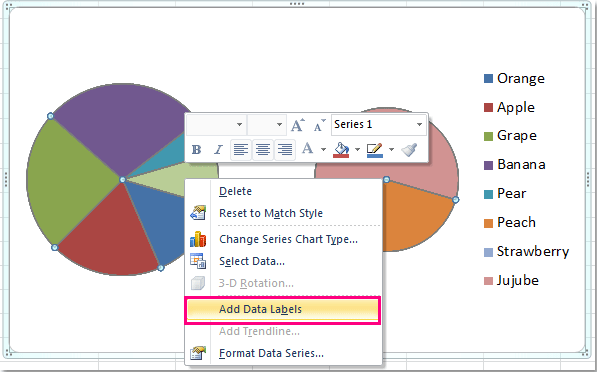
How to create pie of pie or bar of pie chart in Excel?
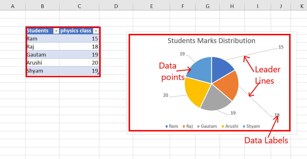
How to Add Leader Lines in Excel? - GeeksforGeeks

How-to Add Label Leader Lines to an Excel Pie Chart - Excel ...
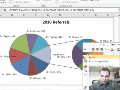
Excel Video 128 Pie of Pie Charts
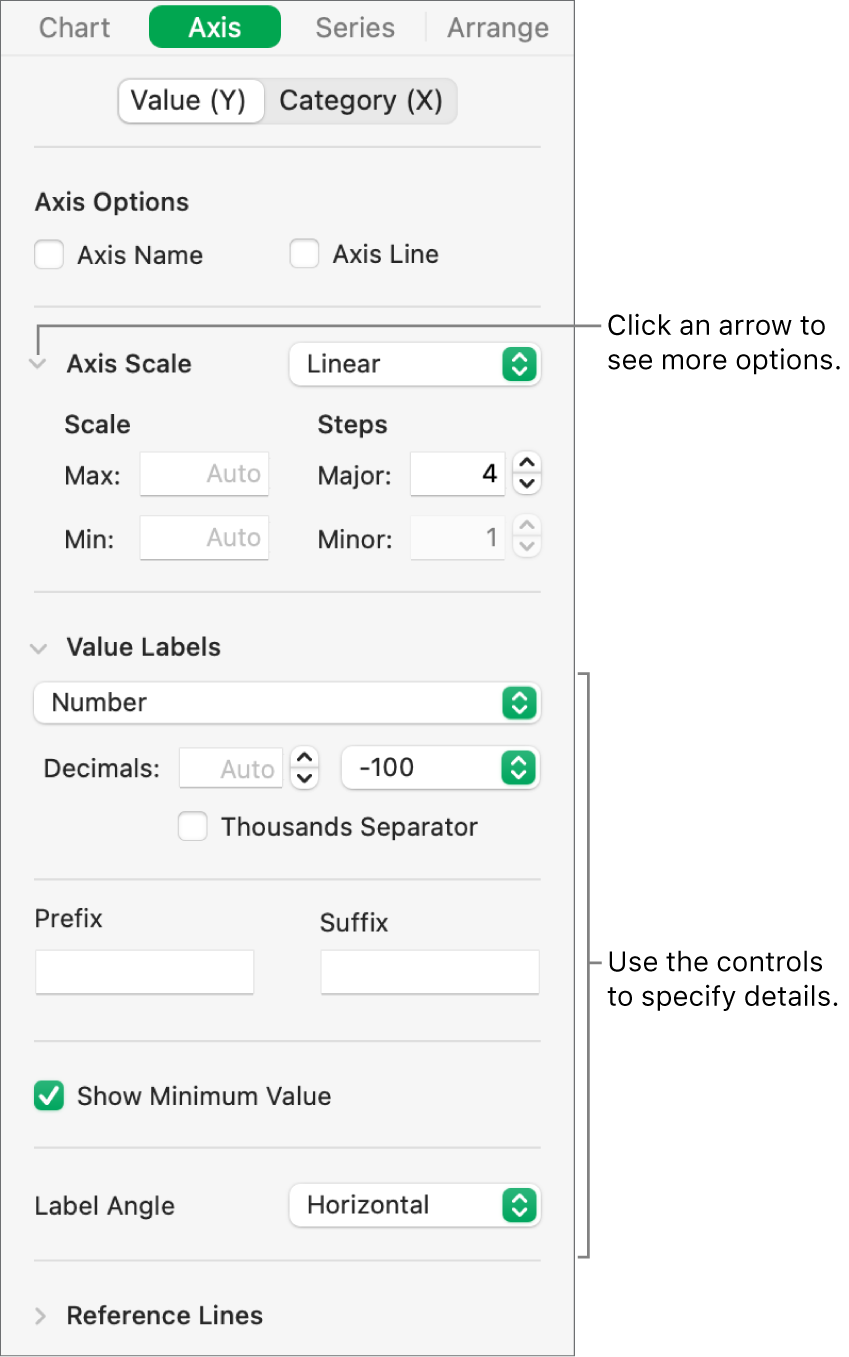
Change the look of chart text and labels in Numbers on Mac ...
/Capture-5c8489fbc9e77c0001422f49.JPG)
How to Create and Format a Pie Chart in Excel
How to Make a Pie Chart in R - Displayr

Change the format of data labels in a chart

How to Show Percentage in Pie Chart in Excel? - GeeksforGeeks

Change the format of data labels in a chart

Formatting data labels and printing pie charts on Excel for ...

How to create pie of pie or bar of pie chart in Excel?

How to make a pie chart in Excel

how to add data labels into Excel graphs — storytelling with data

How to Make a Pie Chart in Excel
How to Make a Pie Chart in Excel
Change the look of chart text and labels in Numbers on Mac ...
How to Edit Legend in Excel | Excelchat
Post a Comment for "42 how to add data labels to a pie chart in excel on mac"