39 excel chart with labels from data

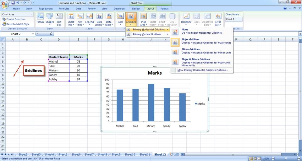
Excel Pivot Table Filter and Label Formatting - Microsoft ... Excel 2016 Images of 2 separate workbooks, each with a data table, pivot table and pivot chart, the one on the right created by copy & paste of the one on the left. The one on the right changed: X axis labels on the pivot chart don't have the multi-level option. Also, unlike the original on the left, there is now a filter button for the chart. support.microsoft.com › en-us › topicHow to use a macro to add labels to data points in an xy ... The labels and values must be laid out in exactly the format described in this article. (The upper-left cell does not have to be cell A1.) To attach text labels to data points in an xy (scatter) chart, follow these steps: On the worksheet that contains the sample data, select the cell range B1:C6.

excelchamps.com › excel-charts › milestone-chartHow to Create a Milestone Chart in Excel in 3 Steps ... Steps to Create a Milestone Chart in Excel. I have split the entire process into three steps to make it easy for you to understand. 1. Set Up Data. You can easily set up your data for this chart. Make sure to arrange your data like below data table.

Excel chart with labels from data

chandoo.org › wp › budget-vs-actual-chart-free-templateFree Budget vs. Actual chart Excel Template - Download May 16, 2018 · Step 10: Add data labels to both lines. Select the lines one at a time (remember, the lines are invisible, so just click where they are supposed to be or use the format box to select them). Now use the + button to add data labels. In older versions of Excel, you need to use either ribbon or menus to add labels. Custom Chart Data Labels In Excel With Formulas Follow the steps below to create the custom data labels. Select the chart label you want to change. In the formula-bar hit = (equals), select the cell reference containing your chart label's data. In this case, the first label is in cell E2. Finally, repeat for all your chart laebls. Excel: How to Create a Bubble Chart with Labels - Statology Then click OK and in the Format Data Labels panel on the right side of the screen, uncheck the box next to Y Value and choose Center as Label Position. The following labels will automatically be added to the bubble chart: Step 4: Customize the Bubble Chart. Lastly, feel free to click on individual elements of the chart to add a title, add axis ...

Excel chart with labels from data. Best Types of Charts in Excel for Data Analysis ... To add a chart to an Excel spreadsheet, follow the steps below: Step-1: Open MS Excel and navigate to the spreadsheet, which contains the data table you want to use for creating a chart. Step-2: Select data for the chart: Step-3: Click on the 'Insert' tab: Step-4: Click on the 'Recommended Charts' button: excel - Formatting Data Labels on a Chart - Stack Overflow sub charttest () activesheet.chartobjects ("chart 6").activate z = 1 with activechart if .charttype = xlline then i = .seriescollection (1).points.count activechart.fullseriescollection (1).datalabels.select for pts = 1 to i activechart.fullseriescollection (1).points (pts).hasdatalabel = true ' make sure all points are visible data … How To Add A Vertical Line To An Excel Chart (2022) Next, you'll likely want to reposition your data label to be directly over your vertical line. To do this, select and right-click on your data label. Click the Format Data Point menu option and the Format Data Label pane should open up. In the Label Position section of the Label Options, select Above. Excel Dynamic Chart Linked with a Drop-down List ... Step 1: Insert the data set into an Excel sheet in the cells as shown above. Step 2: Now select any cell where you want to create the drop-down list for the courses. Step 3: Now click on the Data tab from the top of the Excel window and then click on Data Validation. Step 4: In the Data Validation dialog box : In Allow: Select List.; In Source: Select the cell range for the columns.

How to Print Labels from Excel - Lifewire Select Mailings > Write & Insert Fields > Update Labels . Once you have the Excel spreadsheet and the Word document set up, you can merge the information and print your labels. Click Finish & Merge in the Finish group on the Mailings tab. Click Edit Individual Documents to preview how your printed labels will appear. Select All > OK . How do I make my Data Labels in my Excel chart have a ... Right click on the data label, select "Format Data Labels..." and under "Label Options" check the "Legend Key" checkbox. This will add the little square as it appears on the legend. Share Improve this answer answered Oct 15, 2021 at 19:42 tidus4400 56 1 6 Add a comment Your Answer Post Your Answer How to Add Labels to Scatterplot Points in Excel - Statology Next, click anywhere on the chart until a green plus (+) sign appears in the top right corner. Then click Data Labels, then click More Options… In the Format Data Labels window that appears on the right of the screen, uncheck the box next to Y Value and check the box next to Value From Cells. Bar Chart in Excel - Types, Insertion, Formatting - Excel ... To add Data Labels to the chart, perform the following steps:- Click on the Chart and go to the + icon at the top right corner of the chart. Mark the Data Labels from there After that, select the Horizontal Axis and press the delete key to delete the horizontal axis scale. This is how the chart looks once finished.

Stacked Bar Chart with "different" data labels | MrExcel ... The steps are easy: add data labels to the points, select a set of labels, and click Ctrl+1 to format the labels. In the task pane, check the Value from Cells option. A small dialog pops up, allowing you to select the range that contains your custom labels. Chart Data Label Positioning Macro - excelforum.com Dim mychart As ChartObject Set mychart = ActiveSheet.ChartObjects ("Chart 4") With mychart.Chart.SeriesCollection (1) Dim myvalues myvalues = .Values Dim i As Long For i = LBound (myvalues) To UBound (myvalues) If .Points (i).HasDataLabel And myvalues (i) < 0 And myvalues (i) > -40 Then Selection.Position = xlLabelPositionOutsideEnd - 25 Else Excel Map Chart not showing DATA LABELS for all INDIAN ... Excel Map Chart not showing DATA LABELS for all INDIAN PROVINCES. I've previously posted regarding issues (bugs) with the way the Excel Map chart feature works. I've been putting country risk charts together for a client and I'd like present the data in a map chart. I've found that sometimes it works and sometimes it doesn't requiring you to ... How To Show Two Sets of Data on One Graph in Excel in 8 ... To do so, click and drag your mouse across all the data you want, including the names of the columns and rows. You can check that you selected the data by looking for the cells to be gray instead of white. 3. Click the "Insert" tab and then look at the "Recommended Charts" in the charts group

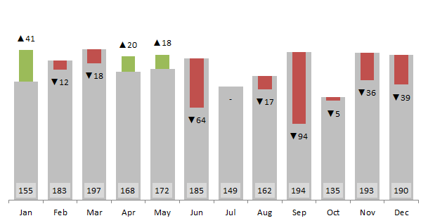
10 ways to present variance analysis reports in Excel - PakAccountants.com

Excel chart labels keep coming back - Microsoft Tech Community Excel chart labels keep coming back I have a data set that I have changed the data labels for to reflect the total count of the objects in a functional category (vertical axes) with the bars of the chart broken up by the material type of the objects in the functional category.

Basic Excel Chart Formatting - MS Excel Charting Tutorial Part 4 | Vertical Horizons

5 New Charts to Visually Display Data in Excel 2019 - dummies Enter the labels and data. Put them in the order you want them to appear in the chart, from top to bottom. You can convert the range to a table to sort it more easily. Select the labels and data and then click Insert → Insert Waterfall, Funnel, Stock, Surface, or Radar Chart → Funnel. Format the chart as desired.

Creating Pie Chart and Adding/Formatting Data Labels (Excel) - YouTube

How to Create and Customize a Treemap Chart in Microsoft Excel Either right-click the chart and pick "Format Chart Area" or double-click the chart to open the sidebar. On Windows, you'll see two handy buttons on the right of your chart when you select it. With these, you can add, remove, and reposition Chart Elements. And you can pick a style or color scheme with the Chart Styles button.

Do My Excel Blog: How to design a multiple clustered bar chart series in Excel

How to Create Charts in Excel: Types & Step by ... - Guru99 Below are the steps to create chart in MS Excel: Open Excel. Enter the data from the sample data table above. Your workbook should now look as follows. To get the desired chart you have to follow the following steps. Select the data you want to represent in graph. Click on INSERT tab from the ribbon. Click on the Column chart drop down button.

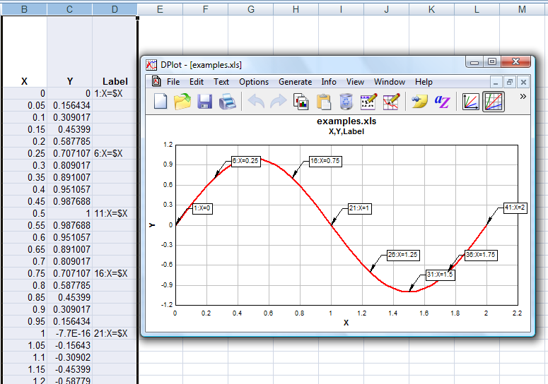
Transferring data > Using the DPlot Interface Add-In for Microsoft Excel > X,Y,Label command

How to Create a Run Chart in Excel (2021 Guide) | 2 Free ... How to Create a Run Chart in Excel Step 1. Calculate the Median Step 2. Build a Line Chart Step 3. Spruce Up Your Run Chart 2 Excel Run Chart Templates 1. Defect Trend Run Chart Template 2. Run Chart with Dynamic Data Labels Run Charts: Overview

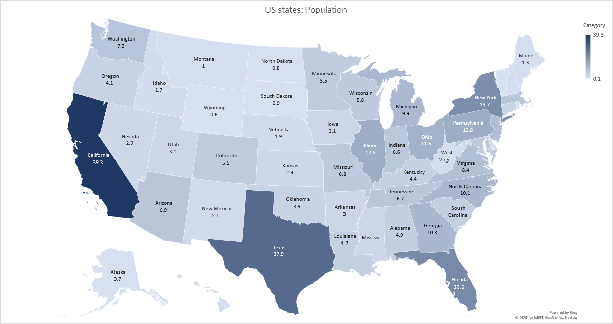
Excel map chart

Chart.ApplyDataLabels method (Excel) | Microsoft Docs For the Chart and Series objects, True if the series has leader lines. Pass a Boolean value to enable or disable the series name for the data label. Pass a Boolean value to enable or disable the category name for the data label. Pass a Boolean value to enable or disable the value for the data label.

How to Create a Geographical Map Chart in Microsoft Excel

superuser.com › questions › 1195816Excel Chart not showing SOME X-axis labels - Super User Apr 05, 2017 · In Excel 2013, select the bar graph or line chart whose axis you're trying to fix. Right click on the chart, select "Format Chart Area..." from the pop up menu. A sidebar will appear on the right side of the screen. On the sidebar, click on "CHART OPTIONS" and select "Horizontal (Category) Axis" from the drop down menu.

Share :